The slides for the following video are shown below:
Slide 1

Welcome to the training course on IBM Scalable Architecture for Financial Reporting, or SAFR. This is Module 18, Extract Time Summarization and Other Functions
Slide 2

Upon completion of this module, you should be able to:
- Describe uses for the Extract-Phase Record Aggregation (formerly knows as Extract-Time Summarization (ETS))
- Read a Logic Table and Trace with ETS views
- Describe how other SAFR functions affect the Logic Table
- Explain the Function Codes used in the example
- Debug ETS and other function views
Slide 3

The prior modules covered the function codes highlighted in blue. Those to be covered in this module are highlighted in yellow.
Slide 4

In the prior module, we learned how the Format Engine creates summarized outputs. Except for producing Standard Extract File formatted records, the Extract Engine typically plays no role in summarization. The one exception is Extract Time Summarization or ETS. With ETS, some level of summarization occurs at extract time.
This can have significant benefits if the final summarized output file is relatively small, but the number of event records required to produce it is very large. This reduces the IO required to write all the detailed extract records, and then for the sort utility to read all those records again. This is a common problem where high level summaries are required for initial analysis of results, before investigating greater detail.
Slide 5

Use of ETS is specified in the View Properties pane, Extract Record Phase Aggregation parameter. The view developer specifies the use of Extract Time Summarization. They also specify how many summarized sort keys the Extract Engine should hold in memory during extract time. Only the sort keys for records held in this buffer at any one time are eligible summarization.
Specifying a large number of records may result in greater summarization during the extract phase. However the Extract Engine allocates memory equal to the number of records multiplied by the number of bytes in each extract record (multiplied by the number of input partitions the view reads when running in parallel mode). If large buffers are specified, or many views use ETS, the Extract Engine may require substantial amounts of memory.
Slide 6

Although ETS collapses some records, complete record aggregation is only assured in the Format Phase. ETS may still result in duplicate records, depending on the order of the input records, because the keys required may overflow the ETS buffer. If the total number of output keys exceed the buffer size, the Extract Engine will dump the record with the least used key to the extract file.
In this example, the ETS record buffer is set to 3 records. However, the total number of output records in the final file will be 4. Because of the order of the input records, the extract file will contain two records with the same key.
Slide 7

After the extract process, the Sort process as part of the Format Phase places all duplicate keyed records next to each other. Thus, no matter the number of duplicates in the Extract File, all be eliminated by during Format Phase processing.
In the example on the left the ETS Buffer is set to 3, and two records with the key AAA 111 are written to the extract file. In the Format Phase these records are summarized together. If the ETS Buffer had been set to 5, memory would have been allocated but never used. If the ETS buffer had been set to 4 no memory will be wasted, and no unnecessary IO will be required.
Slide 8

Consider the following when setting the ETS buffer size:
- The total number of summarized keys in the output file. ETS is often used for thousands and even tens of thousands of rows. However it is not typically used for hundreds of thousands of rows or more.
- The sort order of the input file. If the sort fields for the view are the same as the sort order of the input Event File, then a buffer size of 1 will result in no duplicates in the extract file. This is because once a row is dumped to the extract file the same key will not appear again in the input file.
- The Extract Phase memory available which will be impacted by
- The number of views executing in this Extract Phase
- The memory required for reference tables being joined to by these views
- ETS Buffer sizes specified in other views
- Other items, such as the size of the logic table, buffer sizes for input and output files and Common Key Buffering, etc.
Slide 9

Similar to the Format Phase, ETS only acts upon CT column data for records with the same Sort Key values. However, unlike Format Phase processing with multiple column calculations possible, ETS only performs summarization. Multiplication and division of values is not possible in ETS. Also similar to Format Phase processing, resulting DT values are unpredictable.
In this example the ETS extract file output is only two records, one for “F” and one for “M.” The CT packed values are accumulated to produce the accumulated results.
Slide 10

Although Standard Extract File Format is typically used to send data to the Format Phase, Logical Records can be constructed to read a specific views extract records for additional processing. The ETS output records are often used with SAFR piping to reduce records processed in downstream threads. Piping will be discussed in a later module.
Slide 11

The only change to the Logic Table when ETS is used is the WRXT Write Extract Record function is changed to a WRSU Write Summarized record function. Although a WRXT row can only write one record to the extract file, a WRSU function may write an extract record to the ETS buffer and also a separate overflow record to the extract file if the buffer has overflowed. At the conclusion of Extract Phase processing, all remaining records in the buffer will be dumped to the Extract File. These additional write functions are not shown in the Logic Table trace. The Logic Table trace only shows this function once even though no record or multiple records may have been written to the Extract File.
Next we’ll examine additional Logic Text Keyword functions, and how they impact the Logic Table
Slide 12

SAFR Logic Text Keywords often manipulate the Constant portion of a CFEC or CFLC Compare Field to Constant. For example the BatchDate keyword creates a constant of the execution date. Thus the logic text “Selectif(ORDER_DATE<BATCHDATE())” that is run on January 3, 2010 creates a CFEC comparing ORDER_DATE to the constant “2010-01-03”
Many of the keywords allow math. For example if the Batch Data contains a +3 inside the parenthesis, and were run on the same date the constant would be “20100106” rather than “03”
These function create very efficient processes as constant manipulation is not required during run time. Only the comparison is required.
Slide 13

The Batch Date (also referred to as the “RunDate”) defaults to the system date if not specified in the JCL. It can also set to a specific value as a JCL parameter in GVBMR86. The date is therefore consistent across all views in that execution of GVBMR86.
This date can also be updated in the Logic Table Build program, GVBMR90. This is useful when VDP’s are managed like source code and only created when changes are made to views. In this case the VDP will contain a date for when the VDP was created. These dates can be updated in the Logic Table for the current date by running GVBMR90 in the batch flow and use of the GVBMR90 parameter.
Because processing schedules may provide inconsistent results in rerun situations or when processing near midnight, some installations have written a small program which accesses a enterprise processing table containing a processing date to create this JCL parameter for use by GVBMR86 or GVBMR90. At the end of successful processing this same program then updates the processing date table with the next days date.
Slide 14
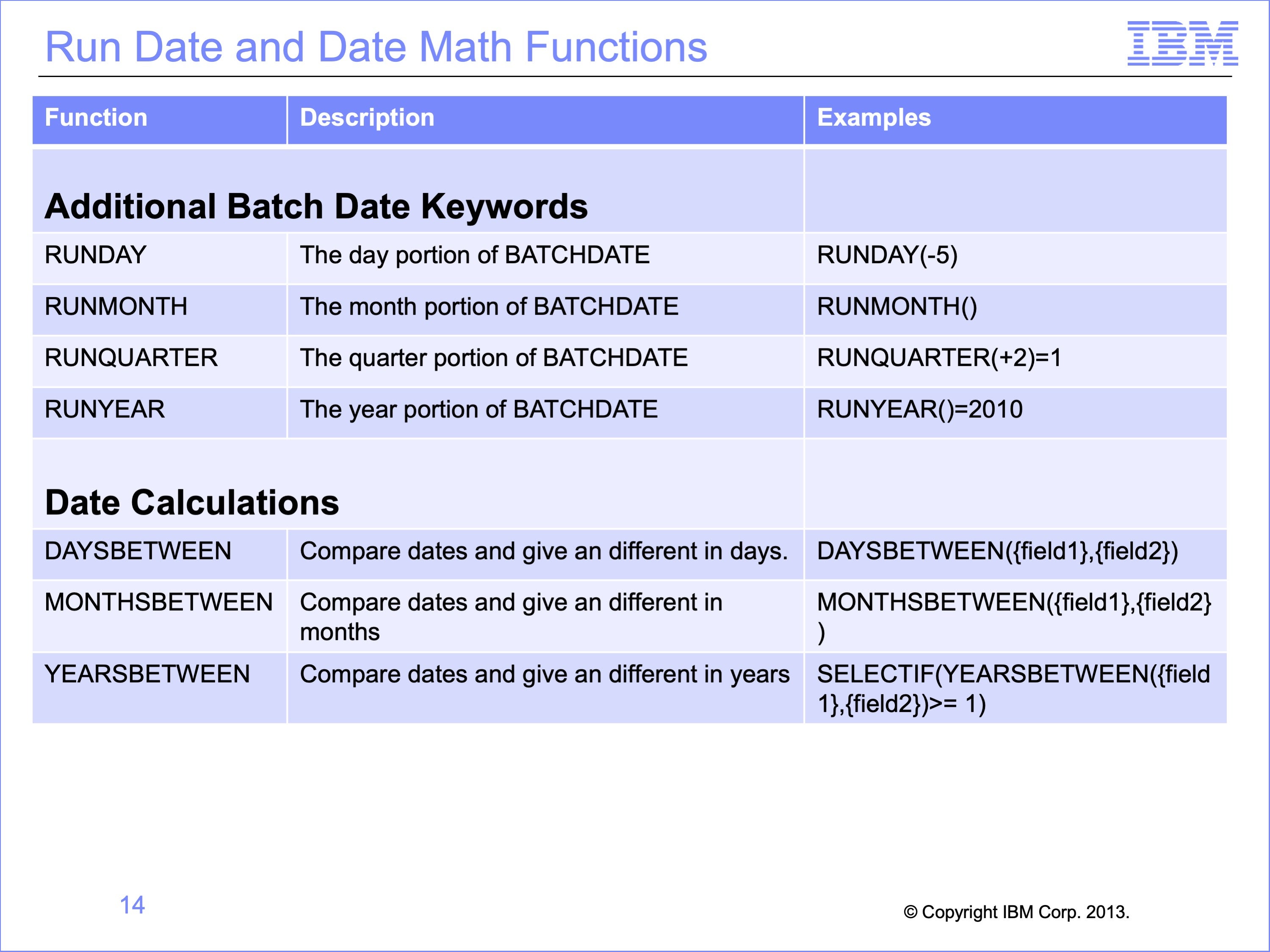
In addition to Batchdate, which returns a full date in CCYYMMDD format, additional key words provide access to a portion of the run date, from day, month, quarter and year. Additionally, each of these keywords allows a numeric parameter which will add or subtract from the current batch date value for use in logic text.
Other keywords allow for calculations and comparisons of dates. Days, months and years between functions performs appropriate date math to return the number of days, months or years. The returned values can be used to evaluate logic text conditions or placed in columns.
Slide 15
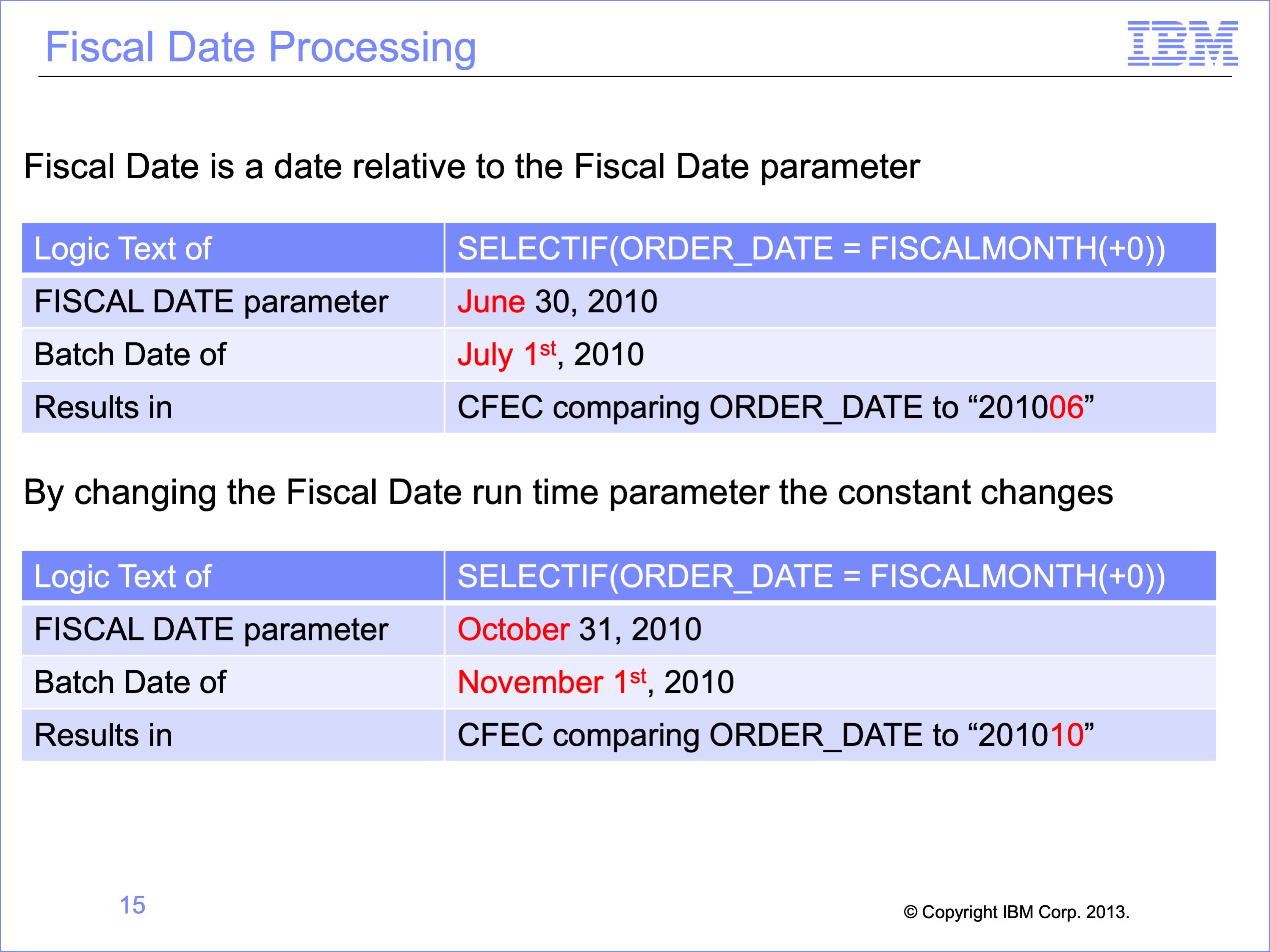
The Fiscal Keywords enable “moving” or “sliding” selection criteria using date criteria. For example, if the view should select data for the current month, the record filters would need to be updated each month as the BATCHDATE value changes. Batch Date returns the month value, for example, a 9, whereas Fiscal Month is a relative month, with “0” meaning “the current month.” Using the Fiscal Date and Control Record, the resolved constant in the Logic Table changes without requiring any changes to the view.
For example, to select data from the current month use the logic text SELECTIF(ORDER_DATE = FISCALMONTH(+0)). When this is executed with a Fiscal Date parameter of June, it results in a constant selecting June records. Without updating the view but changing the Fiscal Data parameter to October results in selection of October records. As the fiscal date constant is updated each month, this effectively creates “moving” criteria for the current month. Attempting to use the BATCHMONTH keyword would require changing the criteria from a value of “6” for June to “10” for October.
Also note that the Fiscal Date parameter is useful when processing on a subsequent day, perhaps passed midnight after all business is closed for the prior day. The Fiscal Date can be set to the prior day or month, recognizing that the data is from the last day of the month, whie the Batch Date reflects when the process was actually run.
Slide 16
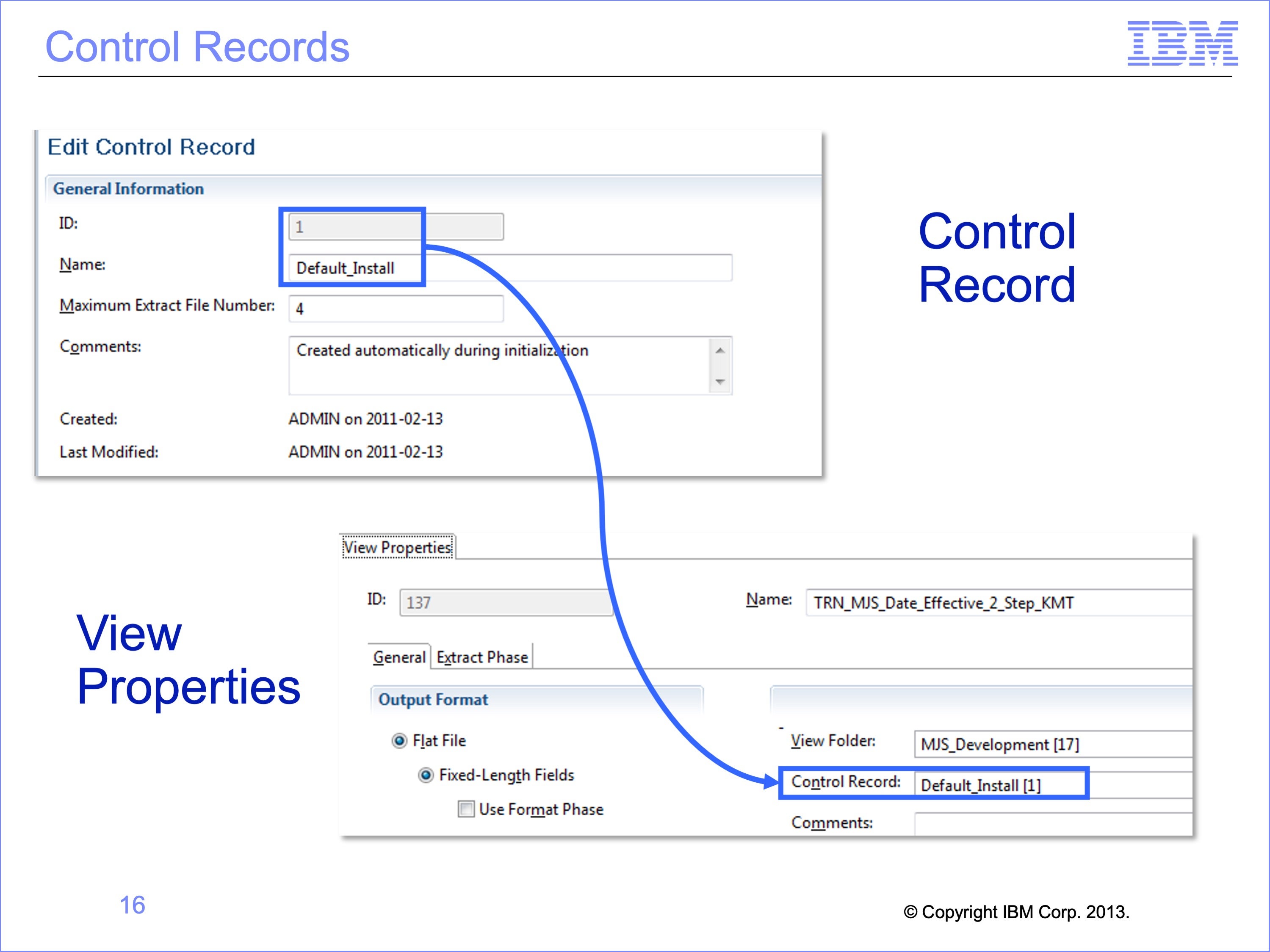
The Fiscal Keywords returns dates based on the fiscal values in the control record for the environment for a view. Each view specifies which control record should be used for its fiscal date processing. This means that different views in the same batch run can have different fiscal dates because they are associated with different control records. This is useful for processing views for multiple companies that have differing fiscal year ends. By comparison, RUNDAY is the same for all views in a batch.
In this example, the view is assigned the Fiscal Date for Control Record ID 1. Other views processed at the same time may be associated with Control Record ID 2.
Slide 17
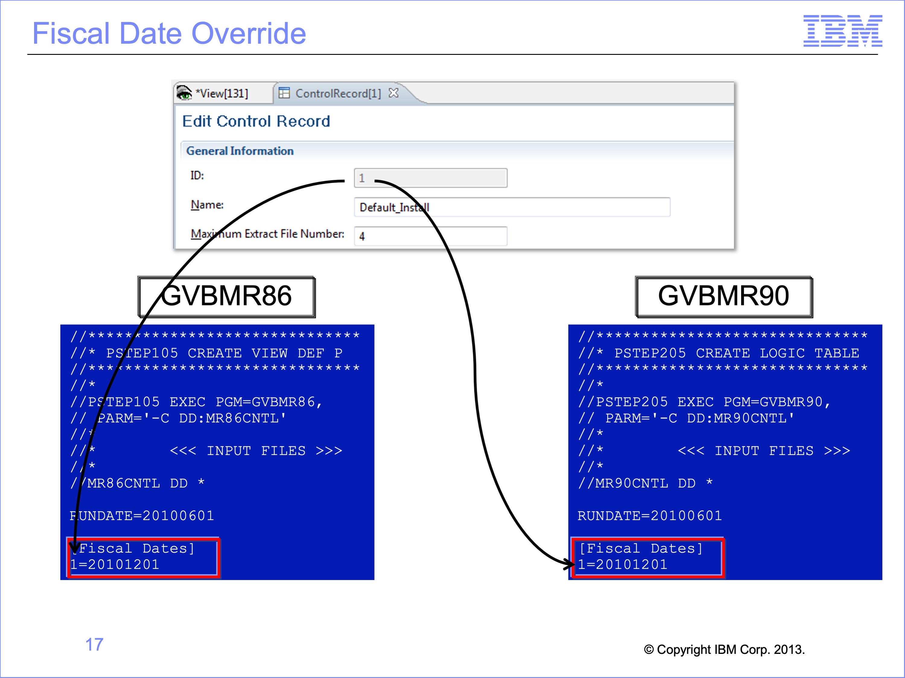
Similar to the Run Date, the actual fiscal date can be overridden in the JCL parameters. To do so, under the keyword “Fiscal Dates” the Control Record ID is followed by an equal sign, and the override date to be used. Multiple dates for different control records can be listed.
Fiscal dates can also be updated through the GVBMR90 parameter for VDP built previously. If no Fiscal Date parameters are passed to either program, they default to the Run Date as the Fiscal Date for any fiscal date keywords.
In this example, the Fiscal Date for Control Record ID 1 is set to 2010-12-01. Note that the Run or Batch Date is set June 1, 2010.
Slide 18
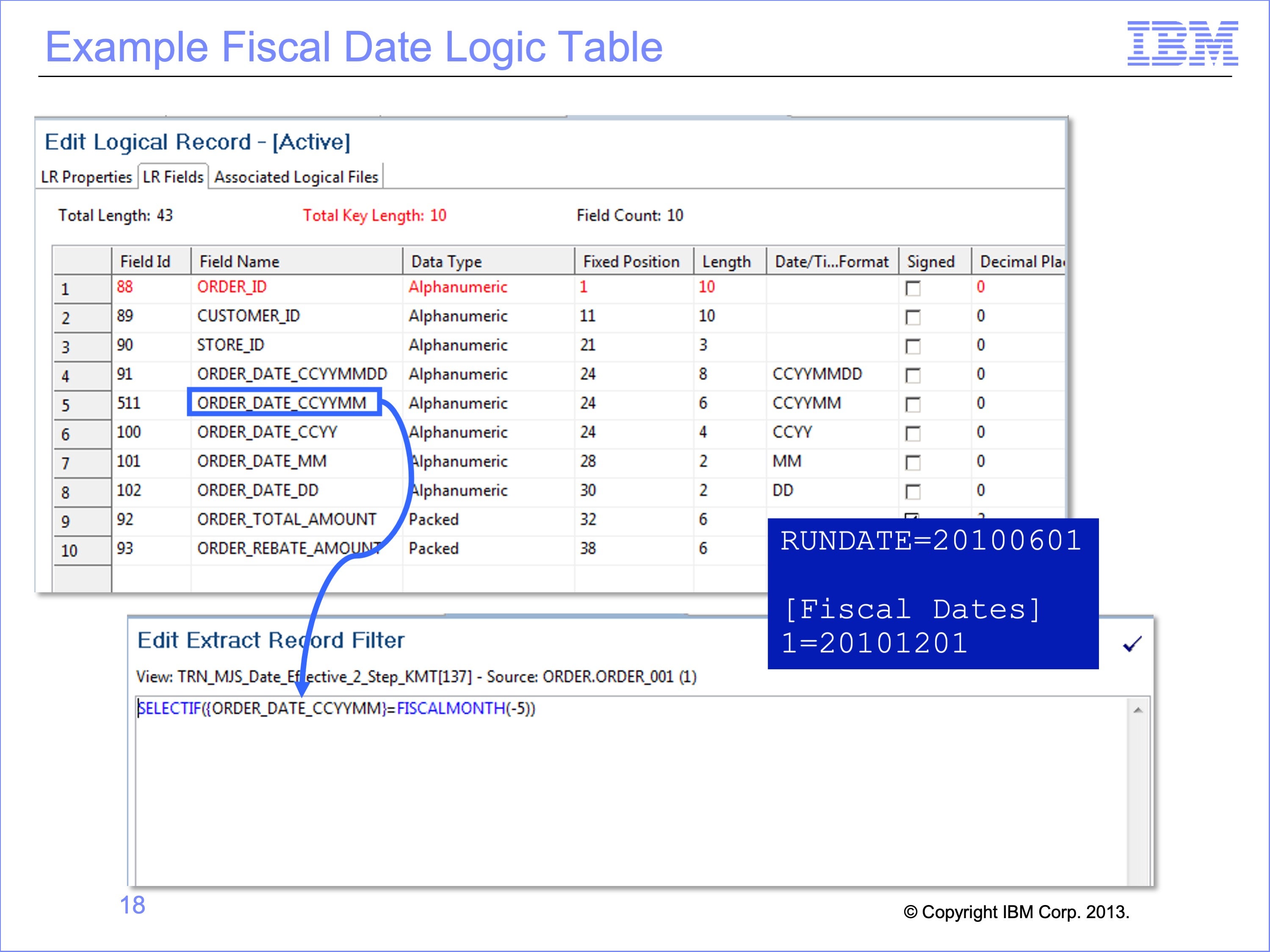
Next we’ll show a logic table containing a resolved fiscal date keyword. In this example, we use the FISCALMONTH keyword, which requires a field in date form with a CCYYMM content code. Our selection logic is SELECTIF(ORDER_DATE_CCYYMM = FISCALMONTH(-5)). The RunDate will be set to 2010-06-01, and Fiscal Date to 2010-12-01. This should result in selecting records from 5 months ago relative to the Fiscal Date parameter passed to GVBMR86, or records from fiscal month 2010-07.
Slide 19
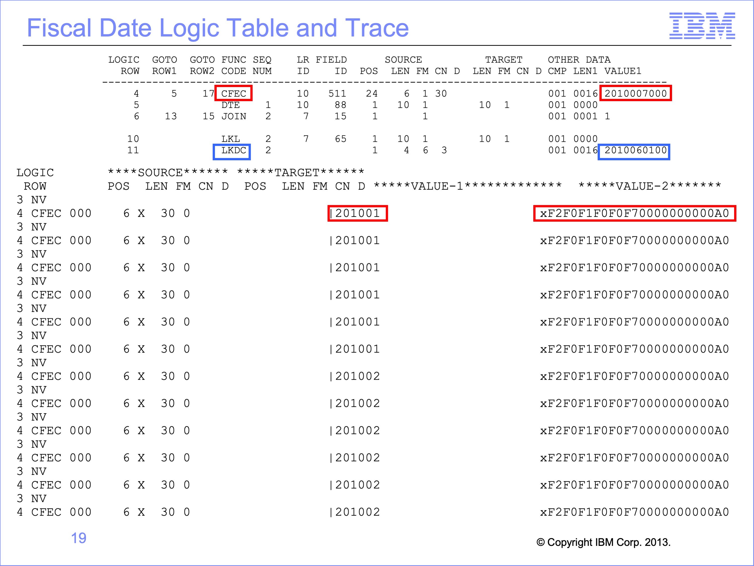
The view logic generates a CFEC function, shown at the top, with the constant of 2010-07 and trailing digits. Because the comparison is only 6 bytes these trailing digits have no impact upon processing. The Logic Table Trace below this shows this value in HEX mode. In this run, all records failed this test.
Note that if they had passed this selection logic, the lookup is effective dated. This can be seen from the LKDC, Lookup Key Date Constant function in the logic table. Note also that this lookup uses the run date, 2010-06, not the fiscal date or the adjusted fiscal date of the Logic Text. This may produce inconsistent results between the selection logic and the date effective join. Care must be taken in creating views to be sure parameters are consistent. Viewing the generated Logic Table can help spot these types of inconsistencies.
Slide 20
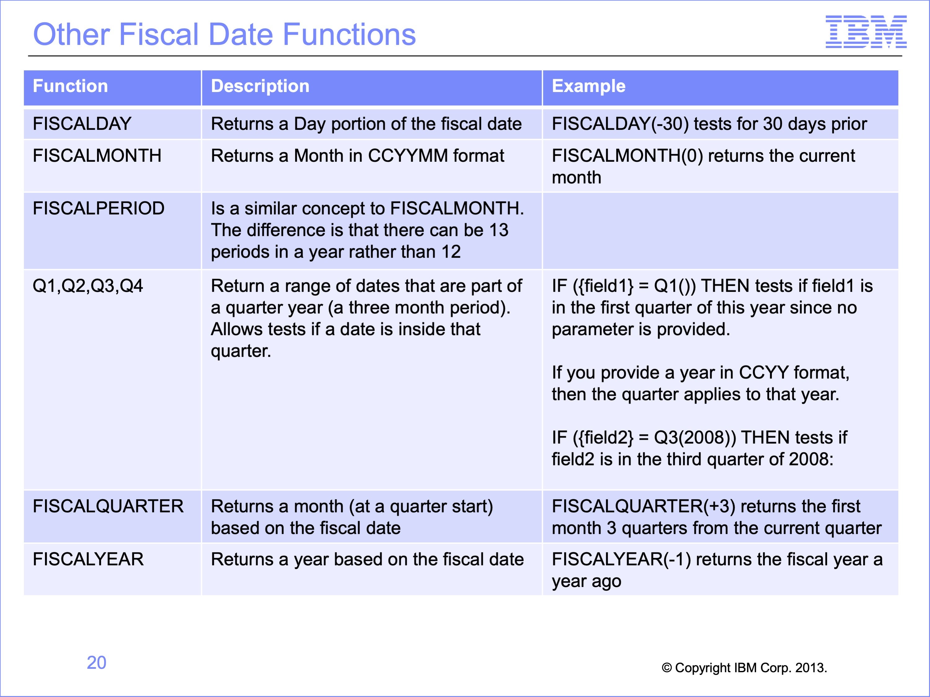
Like BATCH DATE, additional keywords provide access to portions of the fiscal date, including Day, Month, Period, Quarters and Year. These parameters all operate against the Fiscal Date parameter, and can be used in logic text in the view. Each modifies constants in the Logic Table to perform the function. They also allow numeric parameters to perform calendar math, either forwards or backwards.
Slide 21
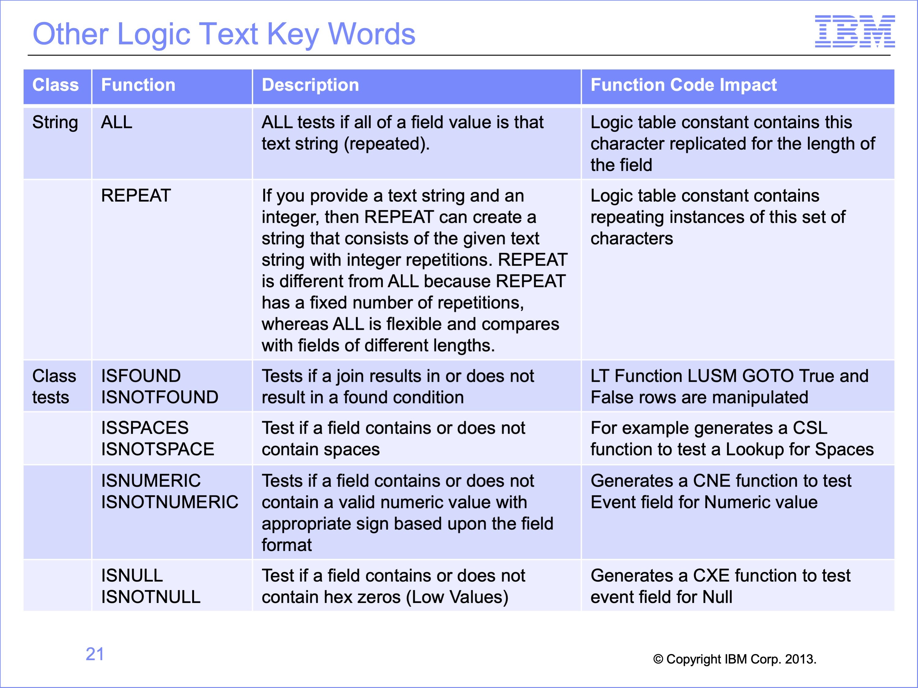
Other Logic Text functions also manipulate the logic table in particular ways. The String keywords of ALL and REPEAT replicate constant parameters in the logic text into constants in the logic table comparison functions. The ISFOUND and ISNOTFOUND functions can change the logic table Goto True and False rows for lookups. Other key words generated specialized logic table functions, like the ISSPACES which generates a CSL logic table function.
Slide 22
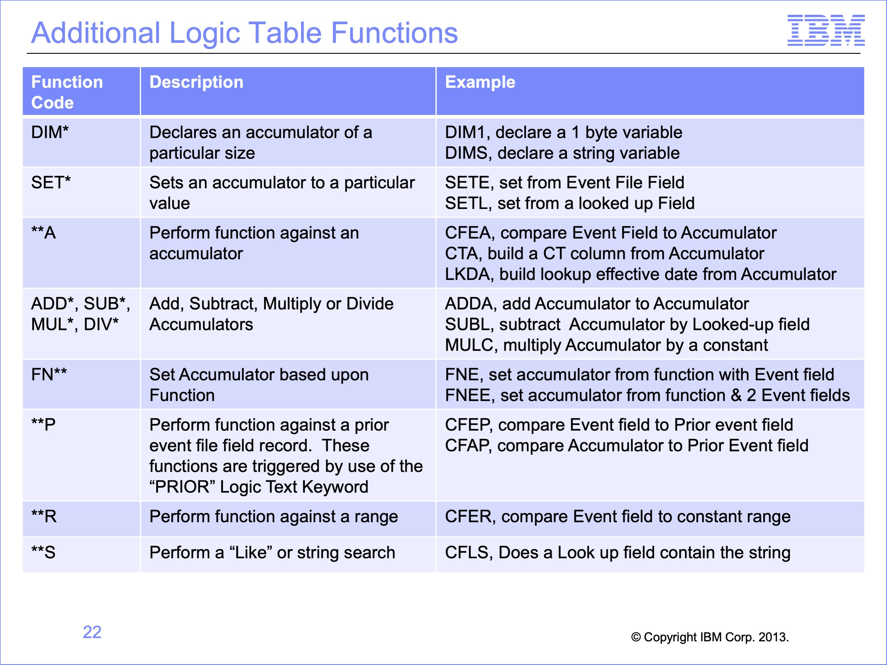
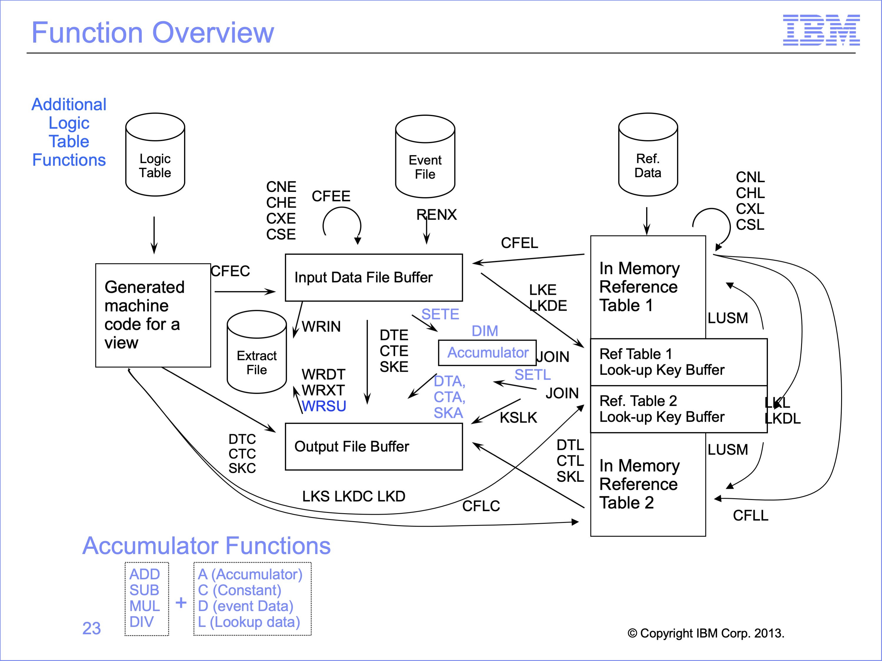
These logic table functions are much less common, but might be seen in logic tables. They perform functions such as declaring accumulator variables, setting those accumulators to values, using them in comparisons and extracting them, and performing math or functions against them. Also logic table functions which work against the prior record might be seen, or range comparisons, or string searches.
Also, if the Logic Text keyword “Begins with” is used, SAFR changes the length of the field being tested to the length of the constant in the logic text. This may result is something like a standard CFEC compare field Event file field to a constant in the Logic Table with the adjust field length.
Slide 23
In this module, we examined the WRSU logic table function, which writes summarized Standard Extract File records. Other less common logic table functions were also introduced.
Slide 24
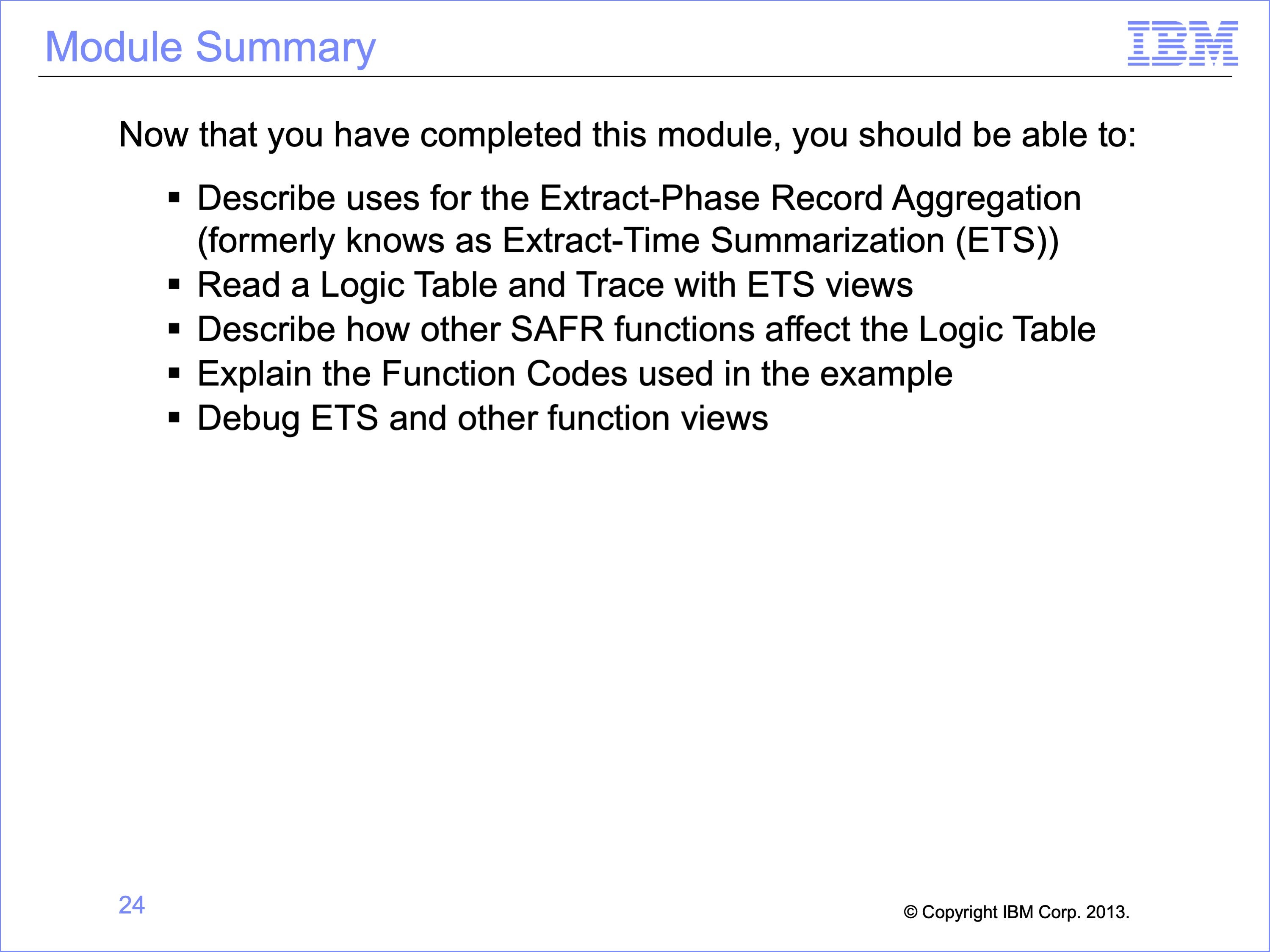
This module described extract time summarization and other logic text keyword functions. Now that you have completed this module, you should be able to:
- Describe uses for the Extract-Phase Record Aggregation (formerly knows as Extract-Time Summarization (ETS))
- Read a Logic Table and Trace with ETS views
- Describe how other SAFR functions affect the Logic Table
- Explain the Function Codes used in the example
- Debug ETS and other function views
Slide 25
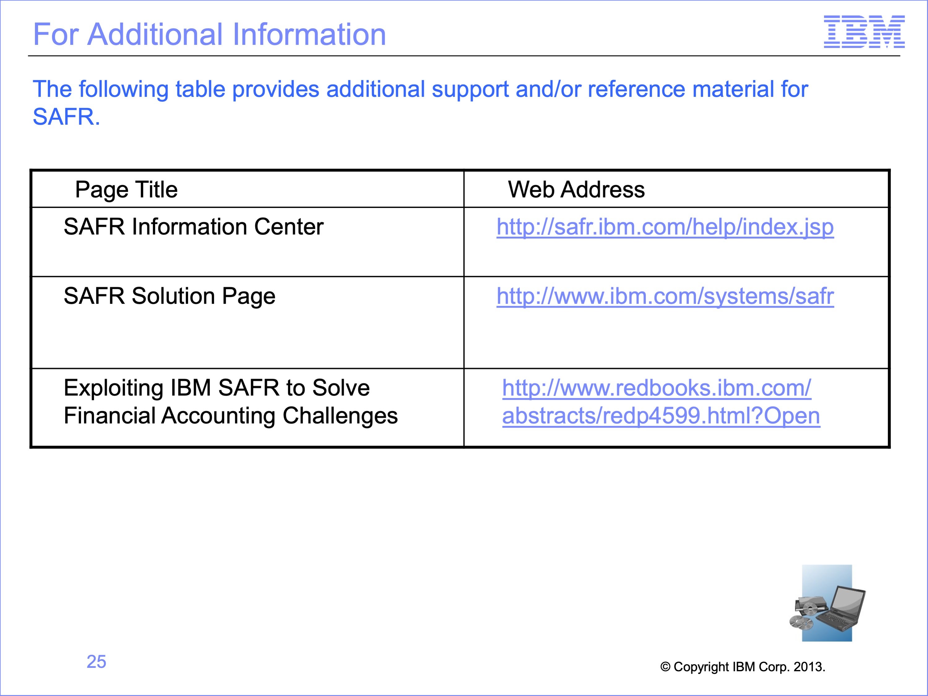
Additional information about SAFR is available at the web addresses shown here. This concludes Module 18, Extract Time Summarization and Other Functions
Slide 26